What it is, and why you should perform it on a routine basis
In order to understand the importance of tympanometry in the hearing care office, it is important to understand oto-immittance. Oto-immittance is the generic term for the procedures that produce measurements of the auditory system as a mechanical system. These include measurements such as acoustic middle ear muscle reflex thresholds, middle ear muscle reflex decay, and other specialized tests, such as Eustachian Tube function tests and physical volume tests. These are all classified under the general rubric of oto-immittance testing.
|
Tympanometry is the first of these oto-immittance procedures typically performed in a hearing care office. Why? Because it is elegant and relatively simple to perform, and it is one of the most informative tests available. However, according to The Hearing Review 2006 Dispenser Survey, only half (50%) of all dispensing offices/practices routinely perform tympanometry during an adult hearing assessment, and a similar survey question in The Hearing Journal revealed that tympanometry was performed “most of the time” or “always” in only 51% of offices/practices.
This article is not intended as a comprehensive instruction manual for performing tympanometry. Rather, it is designed as an introduction for those who do not routinely perform tympanometry, or as a “refresher” for those already versed in this important area of hearing testing.
Why Tympanometry is Useful
Tympanometry is probably the most effective and most efficient test ever devised for evaluating the middle ear system. It is useable with children, adults, and seniors. It is a wonderfully effective and efficient procedure that permits us to get a great deal of high-quality information quickly without any overt effort on the part of the patient (ie, the patient doesn’t have to do anything). In fact, the patient doesn’t even have to be conscious or feeling especially participatory—one more reason why this test is useful and effective, especially for special populations.
Otitis media and pediatric patients. Tympanometry is becoming one of the most common procedures for hearing screening in schools. It is also an efficient screening tool in the offices of pediatricians. In fact, the American Pediatrics Association states that impedance (and, particularly, tympanometry) should be performed to evaluate the health and function of the patient’s middle ear system.
We now recognize that otitis media (OM)—the general term for “middle ear diseases” such as acute or chronic otitis media or otitis media with effusion—is the single most-common health care problem in children. We have also come to recognize that “chronic, recurrent, middle ear disease” can potentially play a significant role in (or lead to) a delay in the acquisition of language—which leads to delays in speech, reading skills, and diminished academic performance.
Adults and medical referrals. Adults may or may not get diagnosed or treated for OM. If they spontaneously recover, the OM may return, and they may experience a long-term cycle of recurrence and recovery. Many adults no longer bother to go for treatment of OM due to the frequency of the problem. It’s also worthwhile to recognize that some seniors tend not to get treated for it.
Conductive hearing problems are defined by the relationship of air-conducted thresholds and bone-conducted thresholds. Let’s talk about what this means at the basic level. When we test someone’s hearing in a clinic, we make several measurements. The first thing we should do, after taking a thorough history and looking at the ear through video otoscopy, is tympanometry. Why? Tympanometry allows us to look at the auditory system as a mechanical system.
Although not necessarily in this order, we should also measure and compare air-conducted thresholds and bone-conducted thresholds. Air-conducted threshold measurements are a measure of how efficient the ear is relative to moving sound through the air. That is, we’re essentially asking, “What is the ear doing?” Bone-conducted thresholds are measurements of the efficiency of sound passage through the bone. That is, we’re essentially asking, “What is the ear capable of doing?”
If the ear is doing as well as it can, then that condition is known as “sensori-neural”—whether the person’s hearing is normal or not normal. “Sensorineural” indicates that air-conducted thresholds equal bone-conducted thresholds; the ear is doing what it is supposed to be doing. However, when conductive problems arise, the ear is not doing everything it is supposed to do. When there is an “air/bone gap” at a given frequency, we say that there is a “loss of efficiency” in that system. In fact, we define conductive loss as a loss of efficiency—or interruption of sound transmission—in the mechanical system of the middle ear.
Notice that hearing has not been mentioned yet. That’s because tympanometry is not dependent upon hearing. In fact, if there is no sensory or neural hearing at all (ie, a “dead ear”), but the mechanical system is still intact and functioning normally, it is possible to get normal tympanograms.
So it is vital for us to understand what we are trying to do with basic tympanometry. A tympanogram is a dynamic measurement of the activity of the tympanic membrane (TM). We generate a specific activity across that membrane, then see what type of pattern the ear exhibits. Researchers and clinicians have provided us with information about what a “normal” pattern looks like and have linked different types of patterns to specific disorders and pathologies. So, when we measure tympanometric responses of an individual’s ear, we gain information about the structures of the ear and/or conditions likely to be causing the interruption of sound transmission.
Most important, tympanometry tells us whether that patient needs to be referred for medical treatment or medical evaluation; it provides a very quick, very accurate, physiologic test that helps us understand the condition of the middle ear.
Tympanometry Basics: Fundamentals of Ear Anatomy and Physiology
To truly understand tympanometry, you need to have knowledge of the anatomy and physiology of the ear and the basic physics of sound.
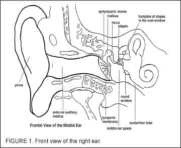
Figure 1 shows a front view of the right ear. On the far left side of the illustration is the auricle (the external ear). Proceeding medially from the concha toward the tympanic membrane is the external auditory meatus, or “ear canal.” The outer third of the ear canal is skin over cartilage, and the inner two-thirds is skin over bone. Within the ear canal, there is very little fatty tissue, but there does exist a highly vascular network, as well as a network of neural end organs (over the bone and under the skin).
The ear canal of most adults is roughly 2.5 cm (about 1 inch) in length from the concha opening to the tympanic membrane, but the canal can vary in diameter over that length from about a half to three-quarters of an inch. The ear canal is not round, but rather ovoid (ie, it changes over its length). The cartilage in the ears of newborns is extremely soft and pliable. It becomes firmer as we age, and in the adult or elderly it can become quite firm or almost hard. If hard, it can be almost immobile; conversely, it can also become so soft that the cartilage falls in on itself—a “collapsed canal”—with almost any kind of pressure.
At the medial end of the ear canal is the TM. The TM is not flat, but rather shaped more like a cone. As you look down the canal toward the TM, the apex of the cone is pointed away from you (ie, the “point” of the cone is the most medial part of the external ear canal). The umbo is located at this “point”.
Attached to the medial surface of the TM are the ossicles: the malleus, incus, and stapes. Trivia buffs can tell you that these are the smallest skeletal bones in the body. However, what most lay people don’t realize is that these bones are fully “adult size” at birth, and therefore consume a large percentage of the space in the middle ear of a newborn. A single drop of fluid in the ear of a newborn may have a major effect on that child, while that same drop of fluid may have little or no effect in the ear of an adult.
The ossicles are not only connected to the medial wall of the TM, but are also connected to, and articulate with, each other. Each of these bones is suspended independently in the middle ear; if you removed one, the others would retain their position. Together, they perform a mechanical system that acts as a Class II lever: the ratio of the “work” that goes in, compared to that of the “work” that goes out, is improved. In this case, the mechanical advantage is 1.5: 1—if you put one unit of energy in (at the TM), you get 1.5 units out (at the footplate of the stapes).
So, when you deliver sound energy to the TM, it passes directly through and into the cochlea. This whole surface is connected to the medial surface of the tympanic membrane and inserts into the oval window. The footplate of the stapes moves in and out of the oval window so that the force exerted on the TM is exerted directly through the oval window (hence, the reason why it is a mechanical lever system).
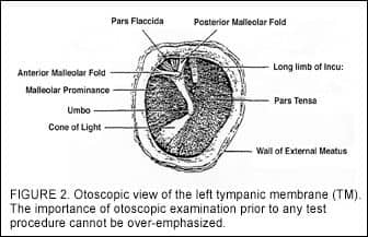
Figure 2 shows an otoscopic view of a left tympanic membrane. The approximate lower 2/3 of the TM is the pars tensa (the “tense part”), and the upper 1/3 is the pars flaccida. There is the annular ring that actually holds the tympanic membrane into the opening in the skull. The superior margin of the umbo is the point on the TM that is most medial (farthest away as you look at it).
Looking through the TM during otoscopic examination, the shadow of the long process of the malleus often can be seen. Sometimes, one can even see a thread-like filament (like a cotton thread) that goes across the upper 1/3 of the TM, called the chorda tympani nerve. This is a branch of the 5th and 7th cranial nerves, which provides the sensation of taste to the anterior 2/3 of the tongue. Additionally, in some people, we can see the “head” of the stapes.
The ability to see this is because the TM in primates is translucent; looking through it is akin to looking through waxed paper. During otoscopy, if you look down the ear canal and see what appears to be a “hole” with only a clear layer over it, you could be looking at a monomeric membrane—a single layer of the normally three layers of the TM.
The outer layer of the TM is epithelial tissue, the inner layer is mucosal tissue, and the medial layer is a fibrous layer with “radial and concentric” fibers. It grows out from the center of the TM, and radiates down the ear canal. If you were to put a dot of permanent ink on the TM, in about a year and a half it would be visible on the external ear.
The medial wall is mucous membrane, similar to the lining of the nose and mouth. A critical characteristic of mucosal membrane tissue is that it absorbs oxygen and exudes fluid to moisten the tissue. All of this is happening in the middle ear. If there is a build-up of fluid, that fluid must go somewhere. The middle ear is a “gravity flow” system that tends to become more efficient the older you get. This is because, in infants and youngsters, the geometry of the Eustachian tube is almost horizontal. Newborns tend to spend a lot of time on their backs, causing the Eustachian tube to be horizontal in two planes—and making the gravity flow system less effective. Interestingly, some studies suggest that children who are breast-fed or who are fed sitting up in an elevated chair (similar to a car seat) have a significantly lower incidence of middle ear disease than children who are fed lying flat on their backs with a bottle.
|
The Quest For the Cone of Light In fact, when a physician shines an otoscope down the ear canal, they are usually looking for this cone of light. When they see it, they know that the ear is intact (ie, in a normal position). The TM can be in the normal position only if there is the normal amount of air in the middle ear space; the only way there can be normal air in the middle ear space is if the Eustachian tube (which is shown on the far right of Figure 1) is functioning normally, connecting the back of the nasal cavity to the middle ear space. In general, if the Eustachian tube is working, then the TM will move. But, if it is not (eg, because of middle ear infection or because swelling of the mucous membrane, etc), the air trapped in the middle ear space will be absorbed by the mucous membrane lining of the middle ear. As the volume of the air diminishes, there is an increasing vacuum in the middle ear space, which sucks the TM inward toward the medial wall of the middle ear. This changes the geometry of the cone, and makes the cone of light disappear. |
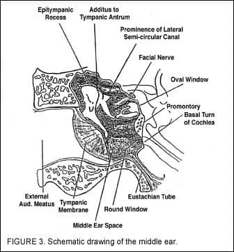
Figure 3 presents a schematic drawing of the middle ear. The key “landmarks” here are the tympanic membrane, the epitympanic recess, the additus of the tympanic antrum (the top of the middle ear space), the three ossicular bones (malleus, incus, stapes), the Eustachian tube, the oval window, and the round window, and the promontory between them.
Sound is introduced through this middle ear system into the inner ear. It is introduced via pressure waves at the oval window membrane by the motion of the footplate of the stapes, which moves in and out of the recess. When the waves are initiated, they are then introduced into the scala vestobuli and travel up the 2 3/4 turns of the cochlea; pass through the helicotrems at the top; and come back down the 2 3/4 turns of the scala tympani. The pressure wave is then released back out into the middle ear space at the round window.
Tympanometry Basics: Auditory Pathways
The portion of the auditory pathway that is involved with oto-immittance and oto-immittance techniques involves the very low portions of the primary auditory pathway of the brainstem. When a signal goes into the cochlea, it must stimulate hair cells and nerve fibers at the base of those cells in order for the signal to be passed along to the brainstem to the temporal lobes. The number of fibers stimulated reaches a critical number, and when it reaches this number, it triggers or “trips” the motor neurons of the 7th cranial nerve. This threshold number is achieved at the acoustic reflex threshold level.
When a critical number of nerve fibers are stimulated, it causes the motor neurons to fire, causing the stapedius muscle of the middle ear to contract. The 5th cranial nerve can also cause the tensor tympani muscle to contract. When the tensor tympani—which is attached to the neck of the malleus and the stapedius that is then attached to the head of the stapes—contracts, its ligaments all contract simultaneously.
When these two contract, they pull the malleus toward the front, and the stapes toward the rear. This turning motion of the ossicular chain causes a loss of efficiency in the motion of the middle ear lever system and results in a conductive loss. There is a “damping” of the lower frequencies which shows up as a low-frequency air/bone gap. That low frequency shift is perceived to shift our own voices downward. This is one reason why our own voices sound different to us in our own heads than it does on a recording. If I record my voice and compare the sounds, my recorded voice is neither down-shifted nor “damped”; it sounds higher because there is no low-frequency air/bone gap.
The portion of the auditory pathway that is involved here is the most primitive part of the auditory pathway. The dorsal and ventral cochlear nucleus are the key landmarks inside the brainstem. The ventral cochlear nucleus is the part through which the acoustic reflex thresholds and the information from the motor-neuron fibers are assessed. From the ventral cochlear nucleus, the signal goes through the trapezoid body (very low in the brainstem) to the medial portion of the superior olivary complex. If there are enough neurons stimulated at the superior olivary complex, then the signal goes to the nucleus of the 7th nerve. When that happens, it triggers the firing of the stapedius nerve and the tensor tympani, “dragging” the ossicle chain out of line, as discussed previously.
Tympanometry Basics: Sound
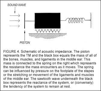
Figure 4 is a representational picture of sound waves striking the TM. The piston moves the mass of all the bones, muscles, and ligaments in the middle ear (represented by the black box in the diagram). This mass is connected to the spring on the right and the piston on the left. The spring represents the resistance the mass encounters as it moves: pressure on the footplate of the stapes, or the stretching or movement of the ligaments and muscles of the middle ear. Finally, the sawtooth wave underneath the black box represents the reactance of the system, or (conversely) the tendency of the system to remain at rest.
This is the inertia—the tendency of a body to remain at rest—that has to be overcome, if the mass is to be set in motion. When hearing care professionals use the word impedance, they are referring to this relationship in the flow of energy. Impedance is the tendency of any system to slow down or impede the flow of energy moving through it. Compliance, on the other hand, refers to the facilitation of the flow of energy through a system. Thus, oto-impedance and oto-compliance are essentially two sides of the same coin.
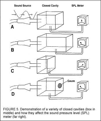
Figure 5a-d shows four boxes into which four identical sound sources are introduced, and a meter allows us to measure the sound pressure level (SPL) within each box. If we put a signal of 85 dB SPL at 226 Hz into a closed cavity of Size 1, it is then possible to adjust the output reading until it reads “0” (ie, the center of the dial of the sound level meter). If you put the same sound into a larger box, the sound pressure will be lower. In Figure 5c, the box is much smaller, making the volume much higher—driving the needle to the right. Finally, if we let some of the sound leak out (Figure 5d), the cavity acts like a larger box, and the sound pressure goes down.
Tympanometry Measurement
In tympanometry, a probe covered with a soft plastic or silicone probe tip is inserted into the ear canal, permitting a hermetic seal to form. This creates a “closed cavity” that resembles a tube with its two ends blocked off: the skin over cartilage (or skin over bone) is the tube, and the ends are the three-layer tympanic membrane (at the medial end) and the probe tip. So, whatever sound is inserted into this cavity essentially stays in this cavity.
On the probe tip are three small holes. Through the first hole we introduce a 85 dB SPL (226 Hz) pure-tone sound; through the second hole we measure the sound pressure in the cavity; through the third hole we create and remove pressure in the cavity to get a dynamic measure of the movement of the TM. By introducing air pressure, we can cause the TM to move. We can exert positive pressure, pushing the TM away from us, or negative pressure, creating a partial vacuum and pulling the TM toward us. We have a limited amount of pressure that can be inserted into an ear when performing tympanometry, and most testing instruments use +200mm H2O to -200mm H2O. How much pressure is this? To give you an idea, a pneumo-otoscope with a little “squeeze” bulb can deliver up to 1000 mm H2O against the TM. So the ±200 mm H2O delivered from the probe tip is not “dangerous” or even seriously uncomfortable for the patient.
While this is not much pressure, it is enough of a range to obtain essential information on the performance of the mechanical system that we’ve been discussing. In basic tympanometry, we insert +200 mm H2O pressure against the TM, effectively pushing it away from us (into the middle ear space). When we do that, we make it “stiffer.” As we make it stiffer, it reflects more sound back into the cavity and this allows less energy (“less sound”) through the TM.
So, the sound is soft when we push the TM away from us. Then, we begin to remove the pressure in the cavity, a bit at a time. As we do, the TM becomes more compliant, lets more sound through, and the perception is that the sound gets louder.
We make a measurement at +200 mm H2O, then remove half the pressure (ie, +100 mm H2O), remove half again (+50 mm H2O), then 0 mm H2O, -50 mm H2O, -100 mm H2O, and finally -200 mm H2O, taking measurements at each point. We plot the amount of sound pressure at each of these points, and connect the dots just like we do with an audiogram; except this time we have plotted a tympanogram.
Each ear is done separately, then they are compared to each other and to our established norms. However, some caution should be applied here. All oto-immittance measurements are based on inferences generated from sound pressure level readings taken in the external ear canal. There is nothing magical about oto-immittance, including tympanometry; they are simply measures inferred from the SPL measurements in the ear canal, between the probe tip and the tympanic membrane.
We also need to recognize that these measurements are made in dB SPL. If you have the kind of equipment that has an earphone on one side and the probe on the other, remember that measurements made with the stimulus tone through the earphone are in dB HL; however, if the stimulus comes (along with the probe tone) through the probe tip, the measurements are in dB SPL.
The bottom line is that we are looking at the dynamic performance of the TM as we exert positive and negative pressures upon it, and the subsequent reactions of the middle ear’s mechanical system in response to TM movement.
What Tympanograms Tell Us
There are several excellent books and publications on tympanometry and interpreting tympanograms. Two of my favorites on the subject are The Handbook of Clinical Impedance1 by James Jerger, PhD, and Selected Readings in Impedance2 by Jerry Northern, PhD. James Hall III, PhD, has also written eloquently on this subject.3 These resources, and other texts, provide a far more detailed explanation of tympanometry than can be offered in this limited space. The following can be viewed as a general outline for how dispensing professionals initially examine a tympanogram.
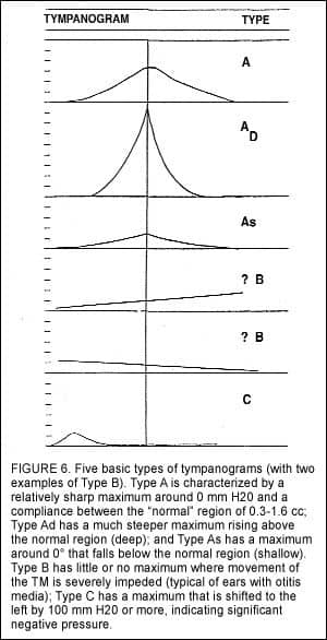
Figure 6 shows the five basic types of tympanograms. The most common is the Type A—the normal characteristic shape for a tympanogram. It is low at both ends (+200 mm and -200 mm H20) and rises, like a tent, to a peak in the middle (centered around 0) and must be between 0.3 cc to 1.6 cc above the base. The Type A tympanogram, generated from a single ear, gives us several vital pieces of information:
1) The eardrum must be intact to get a Type A. If there is a hole in the TM, the pressure will pass through that hole, and you will get a Type B.
2) The TM must be in the normal position. It has to be a cone and function as a cone.
3) There has to be air in the middle ear space to get a TM. In order for there to be air in the middle ear space, the Eustachian tube has to work, along with the intact eardrum, and the normal muscles and ligaments. They have to be intact, they have to be connected, and they have to move through a normal range of motion.
There are two variations of the Type A: the Type As (for shallow or stiff) and the Type Ad (for deep or disarticulated).
A Type As, which looks like an extremely flattened Type A, can be generated by one of two things. Either, there may be ossicular fixation of the bones in the middle ear, or there may be a thickening of the tympanic membrane, which is referred to as tympanosclerosis. Both conditions can impede, or make more shallow, the movement of the TM into the middle ear. White splotchy calcium deposits can also form on the TM, making it heavier—retarding the subsequent movement of the TM or making movement stiffer.
The opposite of this impeded movement of the TM is Type Ad—deeper movement into the middle ear. Like Type As, the TM is intact, but there is an anomaly relative to TM movement. The first and most visible case of Type Ad is the case of the monomeric membrane. This usually stems from a perforation in the TM, over which only a single layer of the “normal skin” grows back. This layer of skin is very thin (as discussed earlier, one can often see through it), very elastic, and essentially inflates when pressurized.
The other cause associated with Type Ad is ossicular discontinuity or disarticulation, which tends to make the TM hypermobile or “floppy.” These types of conditions can result from sporting accidents such as water skiing, as well as from fights or abuse in which the patient has been slapped over the ear or had their ears boxed (cupped hands struck simultaneously over the ears). It is possible for the bones of the middle ear to become broken, or dislodged, and the height and flaccidity of the tympanogram will reflect this abnormal movement.
In addition to the three types of Type As, there are the Type B and Type C tympanograms. The discussion may be facilitated by examining Type C first. The Type C tympanogram has a normal shape and peak, but the peak is shifted to the negative side (ie, the left side of the tympanogram). A Type C is defined as a tympanogram with a peak, where the peak is more negative than -150 mm H2O. In general, we only measure out to -200 mm, so if it is between -150 mm and -200 mm, it is a Type C. This is an ear in transition. Slight negative pressure is fairly common in normal ears, but when the shift equals or exceeds -100 mm, there is reason for concern.
How can you tell if the condition is getting worse or getting better? If you see a Type C and the acoustic reflexes are present, you know it is getting better. If the acoustic reflexes are absent, it is getting worse and becoming a Type B tympanogram.
The Type B represents an ear in which, no matter what you do, you cannot get the TM to move. Type Bs can result from a number of things. The first is that if, when you put the probe tip down the canal, it rests against the canal wall (or a foreign object like wax), and the air pressure of the testing system does not work (ie, no pressure is being exerted on the TM). When this occurs, you get a relatively flat line across the bottom of the graph.
If, on the other hand, you put the probe down into the ear and there is even a very small hole in the TM, the result will be a Type B. The air pressure produced by the probe tip will go right through; instead of pushing against the TM, it is filling the middle ear space (ie, pushing against the medial wall of the middle ear). When this occurs, a flat-line tympanogram will be produced; but now, because of the huge volume, it shows up at the top of the graph. In between the flat line at the bottom and the flat line at the top, there can be other Type Bs that are flat or gradually rising.
If pressure is exerted on an intact TM—this could include fluid, disease, negative pressure so high that the TM is “sucked back” against the medial wall of the middle ear and becomes atelectatic—then the TM cannot move freely. In that case, you also get a Type B. (Author’s Note: There is one variation on this Type B that I have never seen described in the literature which I have witnessed for more than 20 years. It is an “inverted bowl” shape tympanogram: one that starts low, then rises to a rounded top. There is no peak, nor any point; it is just rounded over. Unfortunately, each time I’ve seen this pattern, there has been a cholesteatoma in that ear.)
Some Caveats
Given the above, a tympanogram can be viewed as a mathematical expression, or algebraic sum, of what is occurring in (and on) the middle ear and tympanic membrane. In other words, if you consider the flow of energy through the system, you can add all the positive energy (the pluses) and subtract all the negative energy (the minuses) to arrive at the resultant sum.
This means that, if you had two conditions that produced opposite effects, you could have results that represented the algebraic sum rather than those conditions. For example, if there were a unilateral discontinuity in an ear in which there was also otitis media, the resultant tympanogram could be a Type A—resulting from the Type Ad from the discontinuity and a Type B. However, if you assessed the patient’s acoustic reflexes, you would find that, in this case, they would be gone.
For this reason, tympanograms by themselves aren’t enough. That’s also why, if there is anything at all that is not “perfect” in the complete oto-immittance battery, one always does a complete bone conduction test battery. As noted at the beginning of this article, tympanometry is simply the first of a battery of procedures referred to as otoacoustic immittance measures.
Discussion
At its most basic level, the purpose of screening via tympanometry is to answer the question, “Do I or do I not need to refer this patient for a medical evaluation?” If the patient has Type A tympanograms and his/her acoustic reflexes are present, the question is answered well by the findings. However, if there is an abnormality in the tympanogram, then the indicators are that the patient needs to be referred.
There are cases where an otherwise normal-looking Type A tympanogram will have “notches” (eg, two separate peaks). These reflect the different motions of the TM; the anterior and posterior quadrants move differently. Although this is unusual, it is generally not pathologic. These are Type A, and they do reflect the health of the system.
Acoustic reflex information is critically important here. It is the only way we can know that a patient “hears,” and it gives us an idea of the recruitment in a sensorineural hearing loss by looking at the amplitude of the reflexes. It also provides us with a measurement of the “threshold” of the reflex contraction. This is the level at which the ear “goes non-linear.” Behaviorally, it represents the Loudness Discomfort Level (LDL) at the frequencies (ie, in a hearing aid, this equals the SSPL90).
Tympanograms can also provide insight into fitting hearing aids by understanding the relative “looseness or stiffness of the mechanical system.” For example, when prescribing deeper-fitting (ie, ITE, ITC, or CIC) hearing aids, control of output can become so critical that 2-3 dB at frequencies involving recruitment might mean the difference between success or failure. When controlling the output of a hearing aid, we can take into consideration the height of the tympanogram (ie, volume of the TM’s static compliance). For example, if the tympanogram has a high peak (ie, more mobile TM), it cautions us that we may need to limit the output of the aid. Conversely, when there is a TM through which energy passes less efficiently than normal, we might consider a small addition.
It is also possible to use tympanometry as a tool in loudness validation. To do this, seat the patient 1 meter from a speaker that is located at eye level and at 0° azimuth. You then play “cold running speech” at 60 dB SPL (measured at the ear). Insert the probe that is set to measure reflexes into the “off side” ear, and place the hearing aid into the ear. Finally, adjust the VC until you reach the point where there are no longer reflex peaks (ie, on the peaks of the speech signal). From this point, you can change any parameter in the hearing aid—just as long as you always return to the “Just Not Reflexes” level—and the aid will have the identical “loudness” as perceived by the brain.
Tympanometry is one of the greatest tools we have at our disposal. It has a high level of reliability and repeatability, it gives us important information quickly, and it provides us with fairly easy-to-interpret results. In total, tympanometry takes about 5 minutes for both ears of a patient, and it does not require the patient to be awake or participatory. In fact, in my opinion, the hardest thing about tympanometry involves situating the probe tube or picking the right probe tip to obtain the hermetic seal. If you start doing tympanometry on your next 25 patients, I can virtually guarantee you will never stop using it.
References
1. Jerger J. Handbook of Clinical Impedance Audiometry. Dobbs Ferry, NY: American Electromedics Corp; 1975.
2. Northern JL. Selected Reading in Impedance Audiometry. Dobbs Ferry, NY: American Electromedics Corp; 1976.
3. Hall JW III. Immittance audiometry. Seminars in Hearing 1987;8.
Correspondence can be addressed to HR or Jay B. McSpaden, PhD, PO Box 1043, Jefferson, OR 97352; e-mail: [email protected].